Who Mentions Who in the Office?
This project explores the relationships between different characters in the classic TV show The Office. Using transcript data newly released in Bradley H. Lindblad’s schrute package, I’d like to see who mentions who in the Office. Is one character more popular than the others?
library(schrute)
library(tidyverse)
library(cr)
set_cr_theme()
Let’s take a look at the transcripts:
transcripts <- schrute::theoffice

knitr::kable(transcripts[1:3,])| index | season | episode | episode_name | director | writer | character | text | text_w_direction | imdb_rating | total_votes | air_date |
|---|---|---|---|---|---|---|---|---|---|---|---|
| 1 | 1 | 1 | Pilot | Ken Kwapis | Ricky Gervais;Stephen Merchant;Greg Daniels | Michael | All right Jim. Your quarterlies look very good. How are things at the library? | All right Jim. Your quarterlies look very good. How are things at the library? | 7.6 | 3706 | 2005-03-24 |
| 2 | 1 | 1 | Pilot | Ken Kwapis | Ricky Gervais;Stephen Merchant;Greg Daniels | Jim | Oh, I told you. I couldn’t close it. So… | Oh, I told you. I couldn’t close it. So… | 7.6 | 3706 | 2005-03-24 |
| 3 | 1 | 1 | Pilot | Ken Kwapis | Ricky Gervais;Stephen Merchant;Greg Daniels | Michael | So you’ve come to the master for guidance? Is this what you’re saying, grasshopper? | So you’ve come to the master for guidance? Is this what you’re saying, grasshopper? | 7.6 | 3706 | 2005-03-24 |
By using tidytext, we can split the transcripts into their constituent parts (words).
transcripts_tokenized <- transcripts %>%
  tidytext::unnest_tokens(word, text)

knitr::kable(transcripts_tokenized[1:3,])| index | season | episode | episode_name | director | writer | character | text_w_direction | imdb_rating | total_votes | air_date | word |
|---|---|---|---|---|---|---|---|---|---|---|---|
| 1 | 1 | 1 | Pilot | Ken Kwapis | Ricky Gervais;Stephen Merchant;Greg Daniels | Michael | All right Jim. Your quarterlies look very good. How are things at the library? | 7.6 | 3706 | 2005-03-24 | all |
| 1 | 1 | 1 | Pilot | Ken Kwapis | Ricky Gervais;Stephen Merchant;Greg Daniels | Michael | All right Jim. Your quarterlies look very good. How are things at the library? | 7.6 | 3706 | 2005-03-24 | right |
| 1 | 1 | 1 | Pilot | Ken Kwapis | Ricky Gervais;Stephen Merchant;Greg Daniels | Michael | All right Jim. Your quarterlies look very good. How are things at the library? | 7.6 | 3706 | 2005-03-24 | jim |
We can now use the text to see who mentions who. But first, let’s construct a vector with a list of characters to keep in the analysis. There are 485 characters in the transcripts, so its important we filter only those of relevance:
keep_characters <- transcripts %>%
  group_by(character) %>%
  count() %>%
  arrange(desc(n)) %>%
  head(9) %>%
  pull(character)

knitr::kable(keep_characters)| x |
|---|
| Michael |
| Dwight |
| Jim |
| Pam |
| Andy |
| Angela |
| Kevin |
| Erin |
| Oscar |
This is an optional decision. One may be interested in seeing which characters talk about Jim most, including those characters who are otherwise less relevant. I decide to filter according to the main cast so that comparisons between characters (e.g., through a chord diagram) is feasible.
Who Mentions Who?
Jim: A Case Study
Who is talking to who in the Office?
Now that we have keep_characters, we can filter according to it and spit out who mentions who among the most relevant Office characters.
transcripts_tokenized %>%
  filter(character %in% keep_characters) %>%
  mutate(jim = ifelse(word == "jim", 1, 0)) %>%
  group_by(character) %>%
  summarise(jim = sum(jim)) %>%
  arrange(desc(jim)) %>%
  mutate(character = reorder(character, jim)) %>%
  ggplot(ggplot2::aes(character, jim)) +
  geom_col() +
  coord_flip() +
  fix_bars() +
  labs(title = "Who Mentions Jim?",
       subtitle = "Counts of 'Jim' in The Office Transcripts",
       x = element_blank(),
       y = "Mentions")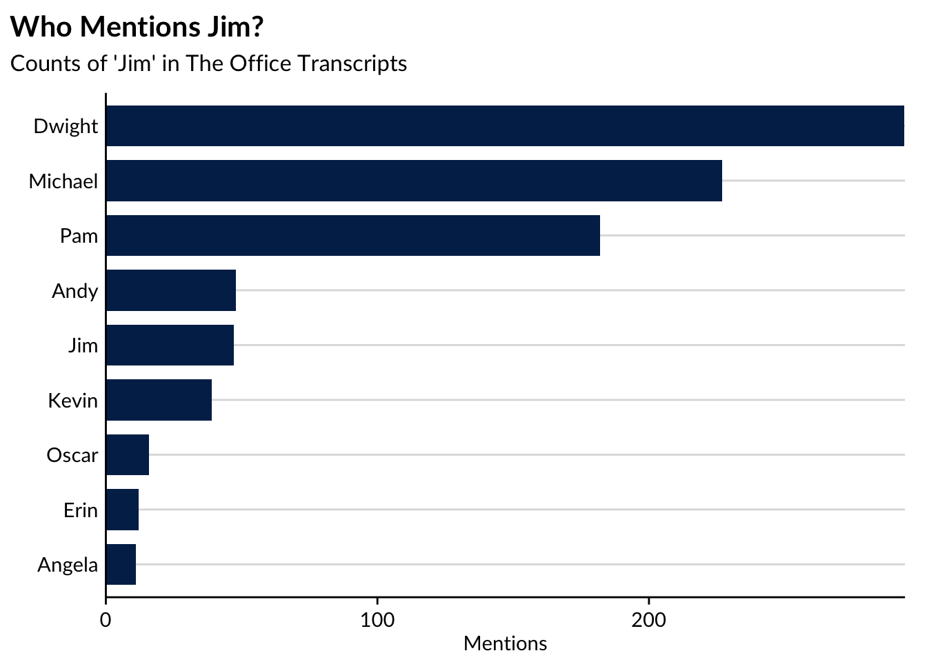
The takeaway here is that Dwight mentions Jim the most, followed by Michael. No surprise there! What I find interesting is that only three characters really talk about/to Jim. After Dwight, Michael, and Pam (and Jim referencing himself, apparently), the mention rate for Jim’s name drops from over 200 to only 60 mentions. It seems as if the writers of the Office intentionally made Jim a subject of conversation among only a few characters!
Replicate for the rest of the cast
Next, we replicate that process for the rest of the cast. There is probably a better way to do this.
data_chord <- transcripts_tokenized %>%
  filter(character %in% keep_characters) %>%
  mutate(jim = ifelse(word == "jim", 1, 0)) %>%
  mutate(michael = ifelse(word == "michael", 1, 0)) %>%
  mutate(dwight = ifelse(word == "dwight", 1, 0)) %>%
  mutate(pam = ifelse(word == "pam", 1, 0)) %>%
  mutate(andy = ifelse(word == "andy", 1, 0)) %>%
  mutate(angela = ifelse(word == "angela", 1, 0)) %>%
  mutate(kevin = ifelse(word == "kevin", 1, 0)) %>%
  mutate(erin = ifelse(word == "erin", 1, 0)) %>%
  mutate(oscar = ifelse(word == "oscar", 1, 0)) %>%
  # mutate(ryan = ifelse(word == "ryan", 1, 0)) %>%
  # mutate(darryl = ifelse(word == "darryl", 1, 0)) %>%
  # mutate(phyllis = ifelse(word == "phyllis", 1, 0)) %>%
  # mutate(kelly = ifelse(word == "kelly", 1, 0)) %>%
  # mutate(toby = ifelse(word == "toby", 1, 0)) %>%
  group_by(character) %>%
  summarise_at(vars(jim:oscar), funs(sum))
Visualize
Now, let’s make a chord diagram!
We first have to convert the data frame into a format chordDiagram will recognize.
circlize_data <- as.data.frame(data_chord) %>%
  pivot_longer(jim:oscar, names_to = "to", values_to = "value") %>%
  rename(from = 'character') %>%
  mutate(to = str_to_title(to))
This process pivots each row of data into a value-key combination, so that the data looks like this:
| from | to | value |
|---|---|---|
| Andy | Jim | 48 |
| Andy | Michael | 40 |
| Andy | Dwight | 80 |
| Andy | Pam | 34 |
| Andy | Andy | 42 |
| Andy | Angela | 33 |
Using that data, we can create a chord diagram quite easily, using a single command from the circlize library. This chapter is helpful.
library(circlize)
chordDiagram(circlize_data, grid.col = c("#B997C7", "#824D99", "#4E78C4", "#57A2AC", "#7EB875", "#D0B541", "#E67F33", "#CE2220", "#521A13"))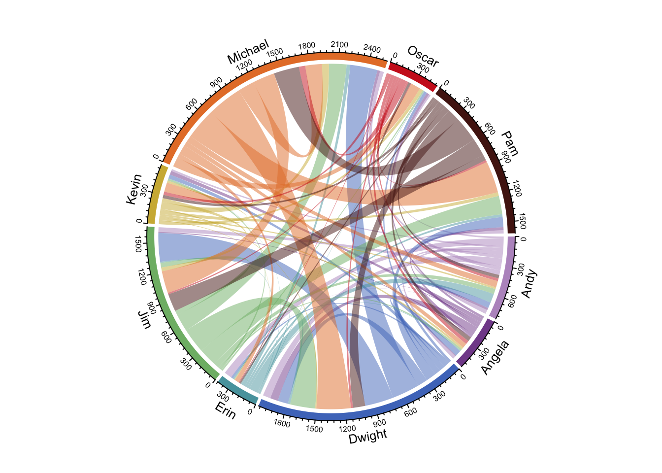
Make It Interactive
With nine people, some of the data can get easily concealed (how often did Angela mention Michael’s name?). One way to fix this is to make the visualization interactive, so that a user can hover over chords to see relationships between characters.
First, we conduct some data cleaning. I found that the rownames and column names have to be of the same order; let’s do a little manipulation to get there:
int_chord <- as.data.frame(data_chord)

rownames(int_chord) <- int_chord$character

row.order <- c("Jim", "Michael", "Dwight", "Pam", "Andy", "Angela", "Kevin", "Erin", "Oscar")
               #, "Ryan", "Darryl", "Phyllis", "Kelly", "Toby")
int_chord <- int_chord[row.order,]
Next, we load Matt Flor’s chorddiag package, and construct a matrix according to its function’s liking:
# devtools::install_github("mattflor/chorddiag")
library(chorddiag)

m <- as.matrix(int_chord[-1])

dimnames(m) <- list(have = int_chord$character,
                    prefer = str_to_title(colnames(int_chord[-1])))
Finally, we add a color palette and construct the diagram.
groupColors <- c("#B997C7", "#824D99", "#4E78C4", "#57A2AC", "#7EB875", "#D0B541", "#E67F33", "#CE2220", "#521A13")

p <- chorddiag(m,
               groupColors = groupColors,
               groupnamePadding = 35,
               tickInterval = 50,
               groupnameFontsize = 12)
p
# save the widget
# library(htmlwidgets)
# saveWidget(p, file="chord_interactive.html")Play around with the diagram here!
Connor Rothschild
Undergraduate at Rice University
I’m a senior at Rice University interested in public policy, data science and their intersection. I’m most passionate about translating complex data into informative and entertaining visualizations.