Texas Vaccination Rates (How to Use Rayshader)
A brief exploration of Texas vaccination rates among kindergartners. Also an attempt to use rayshader for the first time.
Load Packages
library(readxl)
library(tidyverse)
library(stringr)
library(dplyr)
library(ggplot2)
library(ggmap)
library(maps)
library(mapdata)
library(scales)
library(tpltheme)
library(knitr)
conflicted::conflict_prefer("filter", "dplyr")

set_tpl_theme(font = "lato")
Read in Data
tx_vac <- read_excel("data/2018-2019 School Vaccination Coverage Levels - Kindergarten (XLS) .xlsx", skip = 2)

kable(head(tx_vac))| Facility Number | School Type | Facility Name | Facility Address | County | DTP/DTaP/DT/Td | Hepatitis A | Hepatitis B | MMR | Polio | Varicella |
|---|---|---|---|---|---|---|---|---|---|---|
| 9057816000 | Public ISD | A W Brown Leadership Academy | 5701 RED BIRD CTR DR, DALLAS, TX, 75237 | Dallas | 0.8317308 | 0.9086538 | 0.9471154 | 0.8509615 | 0.8413462 | 0.8509615 |
| 9057829000 | Public ISD | A+ Academy | 8225 BRUTON RD, DALLAS, TX, 75217 | Dallas | 1.0000000 | 1.0000000 | 1.0000000 | 0.9909091 | 1.0000000 | 1.0000000 |
| 9109901000 | Public ISD | Abbott ISD | P O BOX 226, ABBOTT, TX, 76621 | Hill | 1.0000000 | 1.0000000 | 1.0000000 | 1.0000000 | 1.0000000 | 1.0000000 |
| 7101130101 | Private School | Abercrombie Academy | 17102 Theiss Mail Road, Spring, TX, 77379 | Harris | 1.0000000 | 1.0000000 | 1.0000000 | 0.7500000 | 1.0000000 | 0.7500000 |
| 9095901000 | Public ISD | Abernathy ISD | 505 7TH ST, ABERNATHY, TX, 79311 | Hale | 1.0000000 | 1.0000000 | 1.0000000 | 1.0000000 | 1.0000000 | 1.0000000 |
| 7101220001 | Private School | Abiding Word Lutheran School | 17123 Red Oak Drive, Houston, TX, 77090 | Harris | 0.7692308 | 0.7692308 | 0.7692308 | 0.7692308 | 0.6923077 | 0.7692308 |
The data contains information on six different vaccines split up by school. The set also contains information on the county of each school, allowing us to aggregate on the county level. By finding the average of the six vaccines listed in this dataset, we can see average vaccination rate by county:
grouped <- tx_vac %>%
  mutate(avgvac = (`DTP/DTaP/DT/Td`+`Hepatitis A`+`Hepatitis B`+MMR+Polio+Varicella)/6) %>%
  group_by(County) %>%
  summarize(avgvac = mean(avgvac, na.rm = TRUE)) %>%
  mutate(County = tolower(County)) %>%
  # rename to subregion so that we can later join with ggplot map data
  rename("subregion" = County) %>%
  filter(subregion != "king")

kable(head(grouped))| subregion | avgvac |
|---|---|
| anderson | 0.9676797 |
| andrews | 0.9715335 |
| angelina | 0.9693150 |
| aransas | 0.9735294 |
| archer | 0.9915167 |
| armstrong | 0.9677419 |
Next, we read in the county-level data from ggplot2 and merge it with our vaccination data:
counties <- map_data("county")
tx_county <- subset(counties, region == "texas")
merged <- left_join(tx_county, grouped, by = "subregion")
Plot
Construct the plot using geom_polygon(), and pay special attention to theme attributes (axes, panels, etc.).
Unfortunately, theme_nothing() led to some conflicts with rayshader, so I essentially recreated it using theme() attributes.
tx <- ggplot(data = merged, mapping = aes(x = long, y = lat, group = group, fill = avgvac*100)) +
coord_fixed(1.3) +
geom_polygon(color = "black") +
labs(fill = "Vaccination Rate") +
#theme_nothing(legend = TRUE) +
theme(legend.title = element_text(),
#legend.key.width = unit(.1, "in"),
panel.border = element_blank(), panel.grid.major = element_blank(),
panel.grid.minor = element_blank(), axis.line = element_blank(),
axis.text.x = element_blank(), axis.text.y = element_blank(),
axis.ticks = element_blank(),
panel.background = element_rect(fill = "white"),
text = element_text(family = "Lato"),
legend.position = "bottom") +
labs(x = element_blank(),
y = element_blank(),
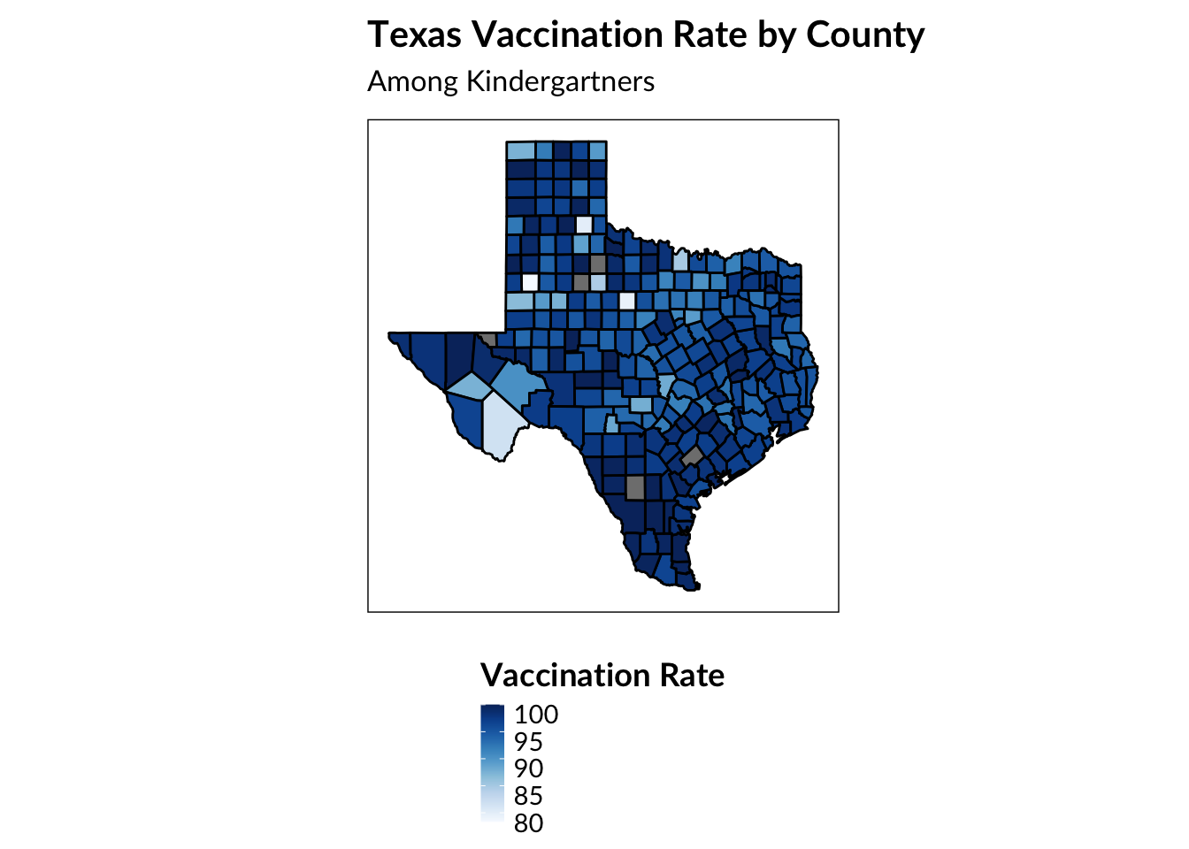
title = "Texas Vaccination Rate by County",
subtitle = "Among Kindergartners") +
tpltheme::scale_fill_continuous()Here’s what the plot looks like before animation:
Rayshader
Load in rayshader and rgl. I’m not sure if rgl is necessary for all R users, but I ran into a few errors on my system (Mac) prior to its installation.
#devtools::install_github("tylermorganwall/rayshader")
library(rgl)
options(rgl.useNULL = FALSE)
library(rayshader)
Lastly, create the plot_gg() object by following the comprehensive documentation on Wall’s README.
par(mfrow = c(1,1))
rayshader::plot_gg(tx, width = 5, raytrace = TRUE, multicore = TRUE, height = 5, scale = 50)

# create custom rotation parameters here
phivechalf = 30 + 60 * 1/(1 + exp(seq(-7, 20, length.out = 180)/2))
phivecfull = c(phivechalf, rev(phivechalf))
thetavec = -90 + 60 * sin(seq(0,359,length.out = 360) * pi/180)
zoomvec = 0.45 + 0.2 * 1/(1 + exp(seq(-5, 20, length.out = 180)))
zoomvecfull = c(zoomvec, rev(zoomvec))

render_movie(filename = "outputs/tx_vac_vid", type = "custom",
frames = 360, phi = phivecfull, zoom = zoomvecfull, theta = thetavec)Connor Rothschild
Undergraduate at Rice University
I’m a senior at Rice University interested in public policy, data science and their intersection. I’m most passionate about translating complex data into informative and entertaining visualizations.