Creating a Streetmap of Springfield, MO

In this post, I expand upon the wonderful Christian Burkhart’s wonderful ggplot2tor tutorial on streetmap creation using ggplot2. My process differs slightly from his in that I include text using geom_label, rather than PowerPoint, to create the text annotations. (This was much more difficult!)

library(tidyverse)
library(gridExtra)
library(grid)
library(ggplot2)
library(lattice)
library(osmdata)
library(sf)

First, per the tutorial, we load street (and river, etc). data:

streets <- getbb("Springfield Missouri")%>%
  opq() %>%
  add_osm_feature(key = "highway", 
                  value = c("motorway", "primary", 
                            "secondary", "tertiary")) %>%
  osmdata_sf()

small_streets <- getbb("Springfield Missouri")%>%
  opq() %>%
  add_osm_feature(key = "highway", 
                  value = c("residential", "living_street",
                            "unclassified",
                            "service", "footway")) %>%
  osmdata_sf()

river <- getbb("Springfield Missouri")%>%
  opq() %>%
  add_osm_feature(key = "waterway", value = "river") %>%
  osmdata_sf()

Next, we define the plot limits, using the lat-long found in the last step.

right = -93.175
left = -93.395
bottom = 37
top = 37.275

In my plot, I’m going to create a text box to hold the city, state, and lat/long combination.

We can create the parameters for this box through some manipulations of the existing plot limits:

top_rect = (top + bottom)/2.0035
bot_rect = bottom + .01
box_height = (top_rect + bot_rect)/2
mid_box = (left + right)/2

Finally, we can create a black and white plot. This follows the same structure as the ggplot2tor tutorial:

plot_bw <- ggplot() +
  geom_sf(data = streets$osm_lines,
          inherit.aes = FALSE,
          color = "#000000",
          size = .3,
          alpha = .8) +
  geom_sf(data = small_streets$osm_lines,
          inherit.aes = FALSE,
          color = "#000000",
          size = .1,
          alpha = .6) +
  geom_sf(data = river$osm_lines,
          inherit.aes = FALSE,
          color = "#000000",
          size = .2,
          alpha = .5) +
  coord_sf(xlim = c(left, right),
           ylim = c(bottom, top),
           expand = FALSE) +
  theme_void() +
  theme(
    plot.background = element_rect(fill = "#FFFFFF"),
    panel.background = element_rect(fill = "#FFFFFF"),
    plot.margin=unit(c(0,-0.5,0,0), "mm")
  )

Finally, we can introduce our text elements using geom_text (as well as borders using geom_rect).

map_bw <- plot_bw +
  # big box
  geom_rect(
    aes(
      xmax = right - .005,
      xmin = left + .005,
      ymin = bottom + .005,
      ymax = top - .005
    ),
    alpha = 0,
    color = "black",
    size = 1
  ) +
  # smaller, label box
  geom_rect(
    aes(
      xmax = right - .01,
      xmin = left + .01,
      ymin = bot_rect,
      ymax = top_rect
    ),
    alpha = .75,
    color = "black",
    fill = "white",
    size = .6
  ) +
  # springfield
  geom_text(
    aes(x = mid_box, y = box_height + .002,
        label = "SPRINGFIELD\n"),
    color = "black",
    family = "Lato",
    fontface = "bold",
    size = 9
  ) +
  # a line that goes behind 'Missouri'
  geom_segment(aes(
    x = left + .03,
    y = (top_rect + bottom) / 2,
    xend = right - .03,
    yend = (top_rect + bottom) / 2
  ), color = "black") +
  # Missouri label
  geom_label(
    aes(x = mid_box, y = box_height - .005,
        label = "MISSOURI"),
    color = "black",
    fill = "white",
    # alpha = .9,
    label.size = 0,
    family = "Lato",
    # fontface = "thin",
    size = 7
  ) +
  # coords
  geom_text(
    aes(x = mid_box, y = box_height - .02,
        label = "37.2090° N / 93.2923° W"),
    color = "black",
    family = "Lato",
    size = 4
  ) +
  # me!
  geom_label(
    aes(
      x = left + .035,
      y = top_rect + .005,
      label = "Design: Connor Rothschild"
    ),
    size = 1.5,
    color = "black",
    fill = "white",
    label.size = 0,
    family = "Lato"
  )

map_bw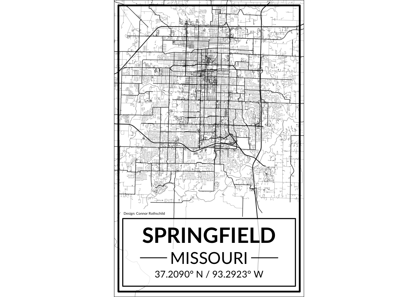

Finally, save the plot:

ggsave(map_bw, filename = "bw_springfield_map.png", width = 3.234, height = 5.016)

Replicate that code with different colors:

plot_gold <- ggplot() +
  geom_sf(
    data = streets$osm_lines,
    inherit.aes = FALSE,
    color = "steelblue",
    size = .3,
    alpha = .8
  ) +
  geom_sf(
    data = small_streets$osm_lines,
    inherit.aes = FALSE,
    color = "#ffbe7f",
    size = .1,
    alpha = .6
  ) +
  geom_sf(
    data = river$osm_lines,
    inherit.aes = FALSE,
    color = "#ffbe7f",
    size = .2,
    alpha = .5
  ) +
  coord_sf(
    xlim = c(left, right),
    ylim = c(bottom, top),
    expand = FALSE
  ) +
  theme_void() +
  theme(
    plot.background = element_rect(fill = "#282828"),
    panel.background = element_rect(fill = "#282828"),
    plot.margin = unit(c(0, -0.5, 0, 0), "mm")
  )

map_gold <- plot_gold +
  geom_rect(
    aes(
      xmax = right - .005,
      xmin = left + .005,
      ymin = bottom + .005,
      ymax = top - .005
    ),
    alpha = 0,
    color = "white",
    size = 1
  ) +
  geom_rect(
    aes(
      xmax = right - .01,
      xmin = left + .01,
      ymin = bot_rect,
      ymax = top_rect
    ),
    alpha = .5,
    color = "#ffbe7f",
    fill = "#282828",
    size = .5
  ) +
  geom_text(
    aes(x = mid_box, y = box_height + .002,
        label = "SPRINGFIELD\n"),
    color = "white",
    family = "Lato",
    fontface = "bold",
    size = 9
  ) +
  geom_segment(aes(
    x = left + .03,
    y = (top_rect + bottom) / 2,
    xend = right - .03,
    yend = (top_rect + bottom) / 2
  ),
  color = "#ffbe7f") +
  geom_label(
    aes(x = mid_box, y = box_height - .005,
        label = "MISSOURI"),
    color = "white",
    fill = "#282828",
    # alpha = .9,
    label.size = 0,
    family = "Lato",
    # fontface = "thin",
    size = 7
  ) +
  geom_text(
    aes(x = mid_box, y = box_height - .02,
        label = "37.2090° N / 93.2923° W"),
    color = "white",
    family = "Lato",
    size = 4
  ) +
  geom_label(
    aes(
      x = left + .035,
      y = top_rect + .005,
      label = "Design: Connor Rothschild"
    ),
    size = 1.5,
    color = "white",
    fill = "#282828",
    label.size = 0,
    family = "Lato"
  )

map_gold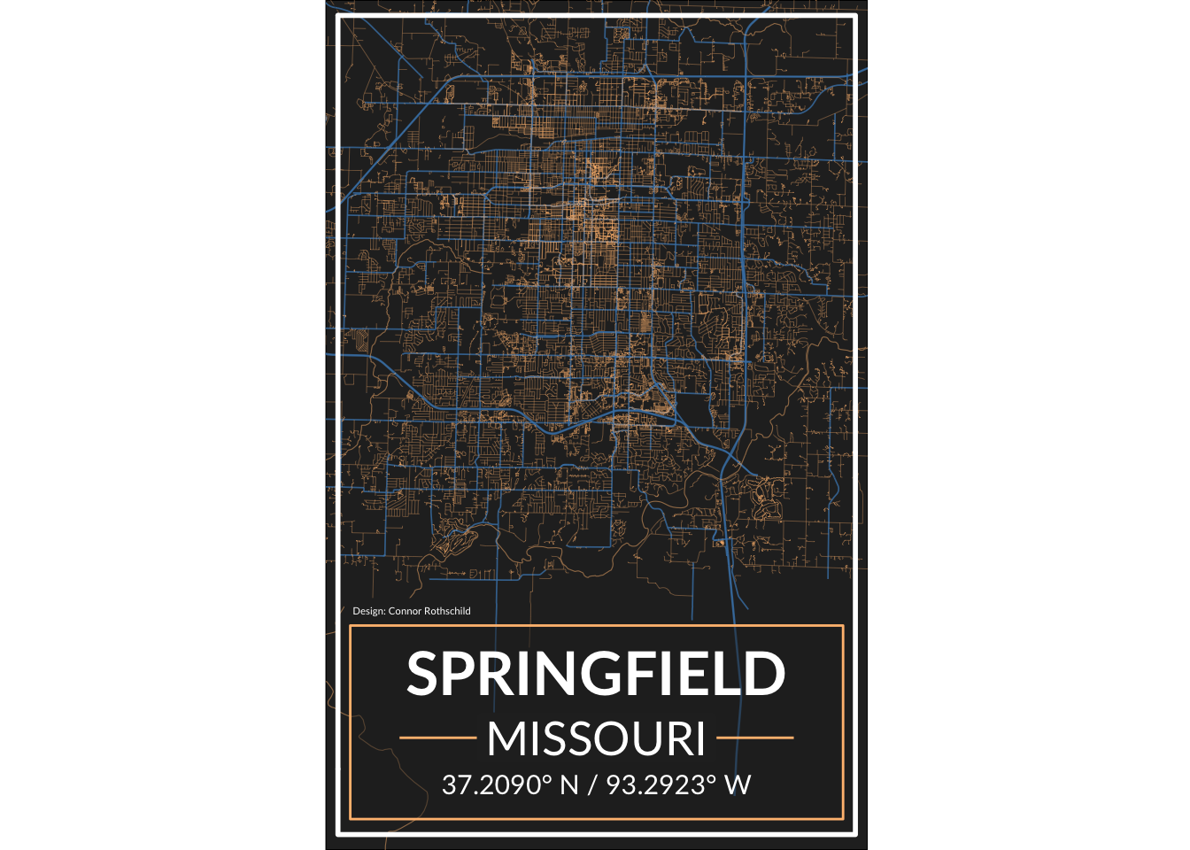

ggsave(map_gold,
       filename = "gold_springfield_map.png",
       width = 3.234,
       height = 5.016)